As the frequency increases, the spring effect of the shaft does not allow the load inertia to accelerate as quickly as the motor which is attached. The shaft starts to twist so that the angle of the load is no longer the same as the angle of the motor. The minimum response will come at an antiresonance frequency where the two masses are moving in opposite directions. The gain of the system then increases with frequency as the main contribution to the load seen by the motor is the torsion of the shaft. This continues up to a resonance at the peak of the curve, after which the inertia of the motor then dominates the load seen by the motor.
Note that his model is simplified, having no damping, whereas real systems have some losses due to material heating when flexing occurs. Adding damping reduces the resonant and antiresonance peaks, but a fairly low loss system will look similar. The electronic model will be a low pass Pi filter, where the torque is modeled as a current, the motor and load inertias are modeled as capacitors, and the spring of the shaft is modeled as an inductor. The value of the inductor is 1/k as a zero-value inductor would represent an infinite stiffness shaft. The motor velocity is Vm, while the load velocity is Vl which would be modeled as voltages in the electronic style model.
We calculate the gain in dB = 20 * log10 (gain), where we are looking at the output velocity versus torque. The frequency scale is plotted on a log10 basis. This allows us to easily look at the gains over a wide range of frequencies.
(These can all be readily modeled in Excel using complex math functions. See sidebar.)
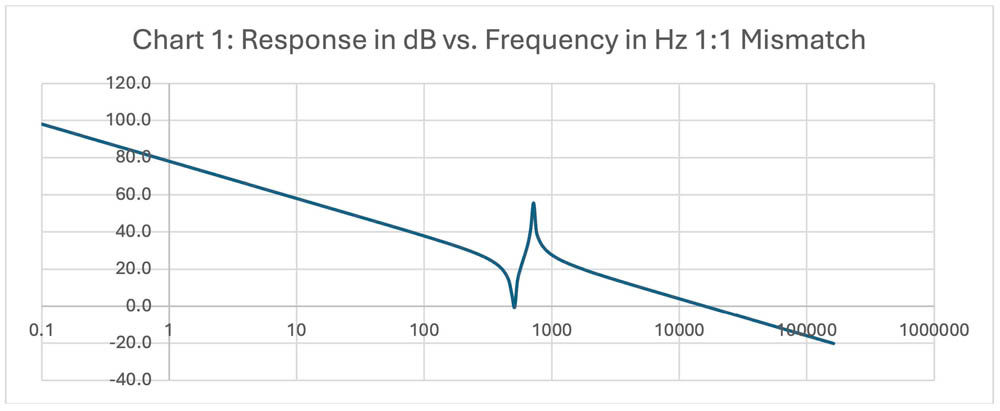
Chart 1 shows the gain for a 1:1 inertial mismatch. The downward peak is the antiresonance. The upward peak is the resonance.

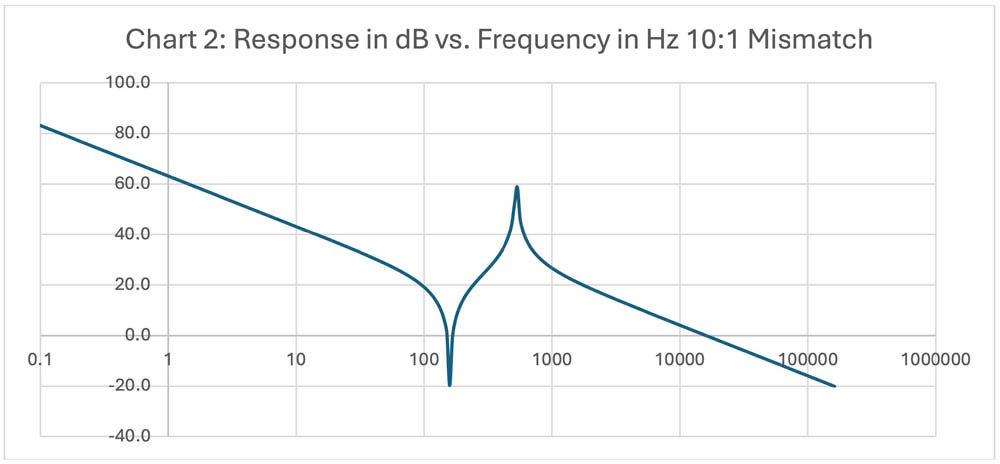
Chart 2 shows the significantly greater gain increase for a 10:1 inertial mismatch
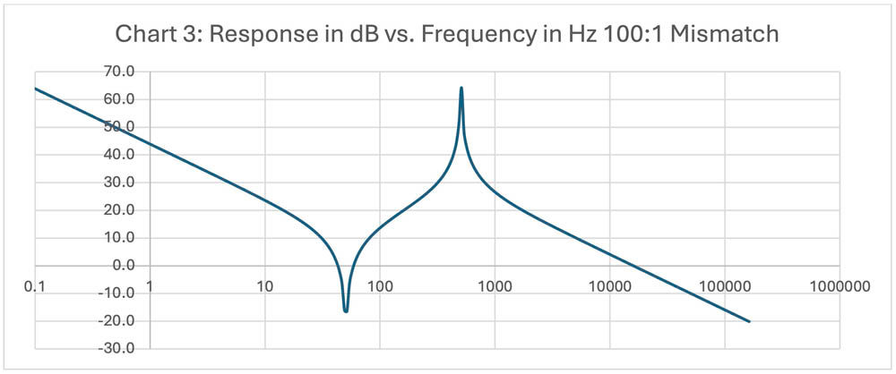
Chart 3 shows the effect for a 100:1 inertia mismatch
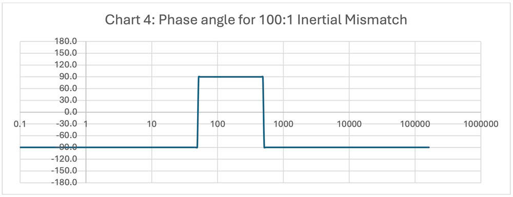
Chart 4 shows the resulting phase angle

You will see in each case the maximum gain from the resonance and the resonance frequency does not change much with the mismatch, as this is mostly determined by the motor inertia and the spring constant of the shaft and coupler. However, the anti-resonance frequency goes down by the square root of (1+inertial mismatch), that is by the square root of the motor plus load inertia.
The low frequency gain drops as 1/(Jm + Jl) that is as 1/total inertia. This is expected as a very large inertial load will accelerate much more slowly than a light inertial load. The control engineer would normally increase the gain of the system to try to make it more responsive.
The problem comes in the upward slope portion of the curve. As the inertial mismatch increases, the gain between the low frequency line (1/(Jm+Jl) and the high frequency line (1/Jm) gets larger, increasing the chance that the system will go into oscillation.
It is also interesting to note that the phase jumps from -90 when the inertia dominates, to +90 when the spring dominates, and back to -90 when the inertia again dominates.
Load Calculations with ExcelExcel can make easy work of load calculations without brushing up on your complex algebra. First you need to enable the complex math by adding the Analysis ToolPak to Excel. This varies with your Excel version, so look up your version. This will add the following functions: COMPLEX: Enter real and imaginary parts of a complex number
IMAGINARY: Extract the Imaginary coefficient
IMREAL: Extract the Real coefficient
IMDIV: Divides complex numbers
IMPRODUCT: Multiplies complex numbers
IMSUB: Subtract complex numbers
IMSUM: Add complex numbers
These few functions allow you to do complex math.
Mechanical loads may be modeled by their electrical analogs.
Torque in N-m => Amps
Rotational velocity in Radians/sec => Volts
Inertia in kg*m2 => Farads
Spring stiffness (N-m)/radian => 1/L (1/Henry)
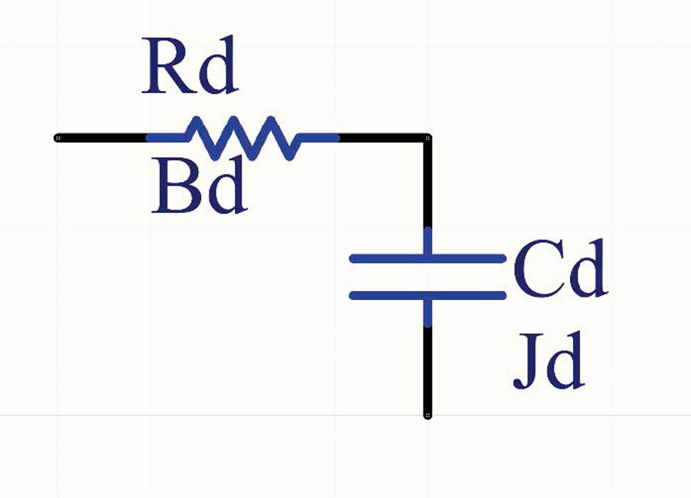
Damper (N-m/radian/sec) => Ohms
A frequency in Hz is transformed to S=j*f*2*PI radians per second
=COMPLEX(0,(2*PI()*B7)) where B7 holds the frequency in Hz
Motor inertia may be modeled as a capacitor C1=J1 , Z1 = 1/(s*C1)
=IMDIV(1,IMPRODUCT(C7,E$1)) where C7 holds s, and E$1 is the first inertia
A shaft torsion (spring) may be modeled as Ls = 1/Ks; Zk=sL
=IMPRODUCT(C7,G$1) where C7 holds x, and G$1 holds L
Load inertia is again modeled as an inertia C2=Jload, Z2= 1/(s*C2)
IMDIV(1,IMPRODUCT(C7,E$2)) where C7 holds s, and E$2 holds load inertia
The total impedance is the parallel connection of Z1 and (Zk + Z2).
If you have impedances Za and Zb in parallel, Zt = 1/(1/Za + 1/Zb)
=IMDIV(1,IMSUM(IMDIV(1,D7),IMDIV(1,IMSUM(E7,F7))))
So starting at the right end, we sum Z2 and Zk, divide it into 1, add it to Z1 divided into 1, and divide this sum into 1. This is the impedance at frequency S in C7, which came from frequency in Hz from B7. |
There are a couple of methods to help stabilize such a high inertial load. The first is to add a low pass filter to the velocity estimator for the control loop. The extra filtering will increase lag in the velocity estimate but will reduce the gain at higher frequencies. This can be considered as making a better estimate of the actual load velocity which continues to reduce with frequency, unlike the sensor on the motor shaft. We can take advantage of the phase boost (+90 degrees) between the antiresonance and resonance frequencies to counter the lag effect of a 2nd order low pass filter to reduce the gain boost associated with the resonance without losing too much phase margin. We will address this in more detail later in this series of articles.
Another method is to add a viscous inertial damper to the motor.


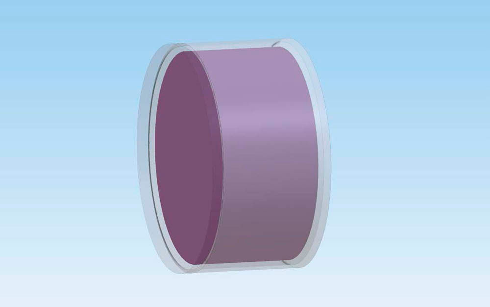
A viscous inertial damper typically has a fairly low inertia housing which contains a higher inertial cylinder which couples to the housing via thick silicone grease. At low accelerations, there is little shear in the grease, and the load looks mostly like a simple inertia. At higher accelerations, the shearing increases, with the inertial damper not significantly moving compared to the input shaft, and the resulting load looking mostly like a like a damper. For a rotary load operating at constant velocity, the inertial load will spin at the same speed as the motor shaft and only a little additional load is introduced. For oscillations in the shaft speed, as the oscillation frequency increases, the shearing of the coupling grease increases, adding damping to the system.
Assuming the housing inertia is low compared to the motor, we can model the shear of the grease as causing a torque to the damper inertia proportional to the difference in radial speed between the case and the damper inertia.
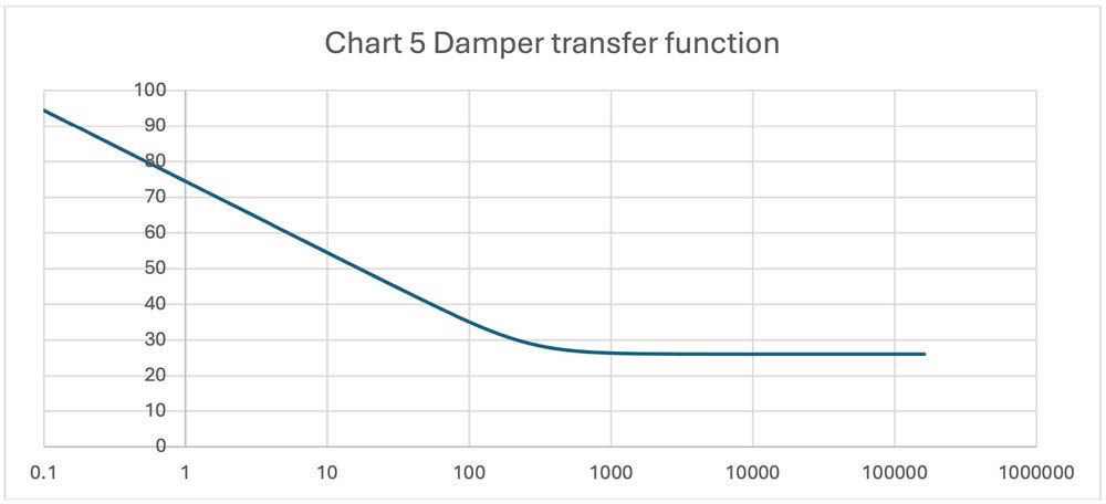
This damper has an inertia about 3x motor inertia, and 1/33 of the load inertia, and the viscous term was adjusted to optimize the shape of the combined curve.
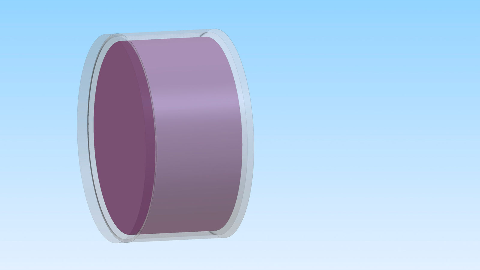
The damper is shown mounted to the motor inertia (stiff compared to the viscous coupling of the grease) with the 100:1 inertia attached to the motor via a shaft
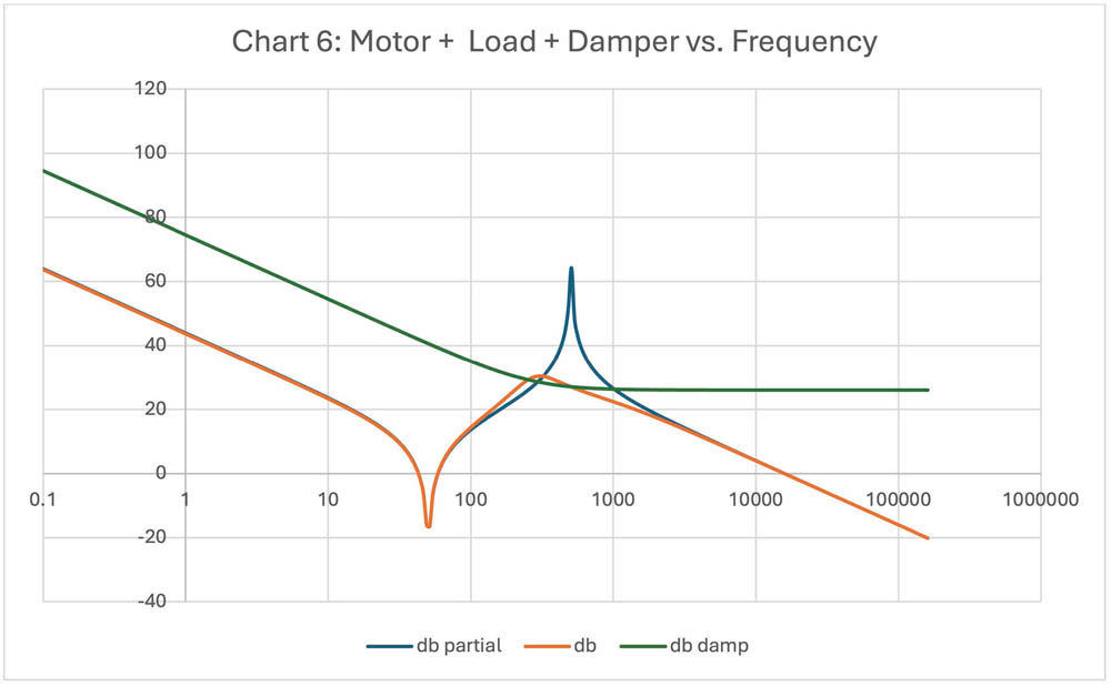
Chart 6 shows the effects when the damper (green) is connected to the motor and 100:1 inertial load (blue) to produce the damped system (orange).
When the damper is placed on the motor shaft, the impedance of the motor with load goes from the dB partial (blue curve) to the dB (orange curve), which has a peak ~ 64 dB down to a peak around 30 dB, almost 64 dB lower. This allows the system gain to be significanlty increased while avoiding oscillations.
This reduced gain spike makes for a system that is much easier to control. Later articles in this series will show how we can produce a similar result electronically in the control system without the need for the mechanical damper.
The charts were all produced in Excel using the complex math function which may be loaded as an extension. This website: https://www.exceldemy.com/learn-excel/math/complex-numbers/ has a nice chart of these functions.
QuickSilverControls.com


