(2)

It has been commonly observed that losses due to air resistance are negligible for circumferential speeds below approximately 20 m/s (Refs. 4, 5). This paper only covers losses due to the fluid’s resistance to the gears and the bearing, ignoring the air’s presence. This loss share covers the previously described churning and squeezing effects and will be addressed as hydraulic losses in this paper.

Although experimental research on the topic of gear power losses has been conducted since mid of the 20th century (Ref. 6) and extensive studies have been made in the following decades (Refs. 7, 8), no general concept has been developed to accurately determine power losses for all components in a transmission. The difficulty stems from the fact that the fluid flow within gearboxes is inherently complex. This is caused by the complexly shaped bodies churning through the lubricant-air mixture. The fluid phenomena for bevel gears are inherently more dynamic than cylindrical gears due to their exposed three-dimensional shape and mounting position. Only a little research on bevel gear churning losses has been conducted. Experimental studies on single rotating bevel gears made by Laruelle et al. (Ref. 4) propose a formulation for the churning torque over filling height, gear radius, and rotational speed for different fluid regimes. Quiban et al. (Ref. 9) updated these formulations and highlighted the phenomena of decreasing churning torques for dynamically varying filling heights. A broad range of tests for different hypoid gears, rotational speed, oils, attitudes, and single and meshing gears have been conducted by Jeon (Ref. 10). This study provides quantitative measurements for a specific gearbox. Therefore, his findings cannot be applied to arbitrary bevel-geared transmissions.

With the advent of high-performance computing and the progress of computational fluid dynamic (CFD) methods, simulations of the motion of the fluid within a gearbox became feasible (Refs. 11, 12). Subsequently, it was demonstrated that CFD is capable of accurately reproducing the fluid dynamics observed in experiments (Ref. 13). The investigations of the last decades are based on traditional CFD approaches that utilize a grid-based Eulerian technique. These methods are established but have to cope with major difficulties: With increasing complexity, that is more moving geometries, narrow gaps, and large geometry curvature, generating a sophisticated computational grid becomes difficult (Refs. 14, 15). Tracking the complex phase interface between air and oil requires a sufficiently fine mesh and the transient deformation of the domain with its moving parts requires adapting the grid over time. These demands raise the computational effort drastically. A variety of mesh and geometry handling techniques are employed to cope with this matter. A summary is given in Concli and Gorla (Ref. 16) and Concli et al. (Ref. 15). However, these methods have been proven to reliably predict churning losses in gears (Refs. 12, 13, 15). A sophisticated overview of state-of-the-art CFD research in numerical drivetrain lubrication applications is given in Maccioni and Concli (Ref. 17). It is carved out that individual methods exist to address hydraulic losses in bearings, gearsets, or pumps individually with more than 80 percent agreement between simulation and experiment. However, most of those papers focus solely on one of those mechanical components per simulation. Considering grid-based methods, e.g., Peng et al. (Ref. 18) presented qualitative results of an automotive rear axle gearbox with rotating bearings and validated their method with experimental values in a specialized test rig considering gears only. Oil, operating conditions, and filling heights are comparable to this paper. The simulation domain was separated into individual mesh zones, where motions were applied by user-defined functions. No detailed assessment of the bearing-induced churning losses is presented.

Smoothed Particle Hydrodynamics (SPH) is a Lagrangian CFD technique that has lower demands on geometry quality, thus decreasing simulation preparation time drastically. Mathematically, this approach renders a moving and deforming grid method where the collocation points are commonly called particles. Since neighboring relationships are updated after advecting the particles no computational grid is required. Here, particles of distinct fluid types represent individual phases and the unique particle type implicitly reconstructs the phase interface. Apart from the native handling of free surface flows, SPH has also proven to provide computational advantages for drivetrain simulations. Keller et al. (Ref. 19), as well as Maier et al. (Ref. 20), conducted SPH simulations 20–25 times faster than a Eulerian simulation of the same problem. These aspects indicate the significant potential of the SPH method in the field of transmission CFD. Being mesh-free, it simplifies the time-consuming geometry preparation and the simulation itself, by making typical procedures such as remeshing or gear-scaling obsolete. Although overall fluid flow was reproduced accurately (Refs. 21–24) this method has not yet been proven to replicate the measured churning losses for various cases with an accuracy of over 80 percent (Refs. 17, 22). The main reason lies in under-resolving pressure gradients in the contacting areas and velocity gradients in churning regions. Multiple approaches with artificially increased fluid-wall friction are employed to calibrate results closer to the experimentally expected values. Contrary to the previous papers, the utilized SPH solver comes with the following differences:

It imposes the boundary-particle interaction by considering the shape of the boundary, i.e., evaluating the boundary integral of the particle’s kernel with the solid wall to ensure consistency of the kernel integration scheme. This is not ensured by employing dummy boundary particles or polygonal wall-distance-force functions (Refs. 25, 26) are used to describe the interaction of the fluid with the wall, which will inevitably lead to substantial spatial resolution dependencies.

• Using multiple particle resolutions per simulation to improve resolving the pressure gradients and fluid boundary layers.
• No usage of artificially increased forces between fluid-wall and fluid-fluid interaction to calibrate results to experimental data.

Moving particle semi-implicit (MPS) characterizes another Lagrangian CFD method. Both MPS and SPH are very similar in their numerical approach as shown in Soute-Iglesias et al. (Ref. 27). Again, multiple studies report accurate prediction of visual oil distribution within gearboxes (Ref. 25, 28). The churning loss determined by applying the MPS method on a high-speed railway system is qualitatively investigated in a similar study conducted by Deng et al. (Ref. 29) as well as in Shao et al. (Ref. 26). A similar qualitative study is presented in Singh et al. (Ref. 24). The results presented are derived from an implicit MPS solver that allows for theoretically larger time steps than the explicit SPH solver in this paper. However, implicit solvers have the disadvantage of solving the pressure Poisson equation by a computationally costly matrix inversion. Additionally, presented hydraulic losses for bearings were reported to be negligible low, i.e. one to two orders of magnitude smaller than the gear-induced hydraulic losses.

This paper outlines a methodology for investigating churning losses of gears and bearings simultaneously in an industrial gearbox by bridging the fluid scale differences with particle-refinement techniques in SPH and subsystem investigations of the bearings. A special focus is set on the importance of replicating the roller bearing’s motion correctly instead of a simple rigid rotation. The method is applied as a parameter study considering rotational speed, turning direction, and filling height to highlight the benefits of cloud-native high-performance computing for virtually replicating experimental test rigs to derive a reliable system response within a few days without building a prototype.

Numerical Approach

SPH Kernel Interpolation

Fundamental to the SPH method is the spatially discrete representation of a continuum with so-called particles. These collocation points, which move along their trajectories, inherit the physical properties of the continuum.

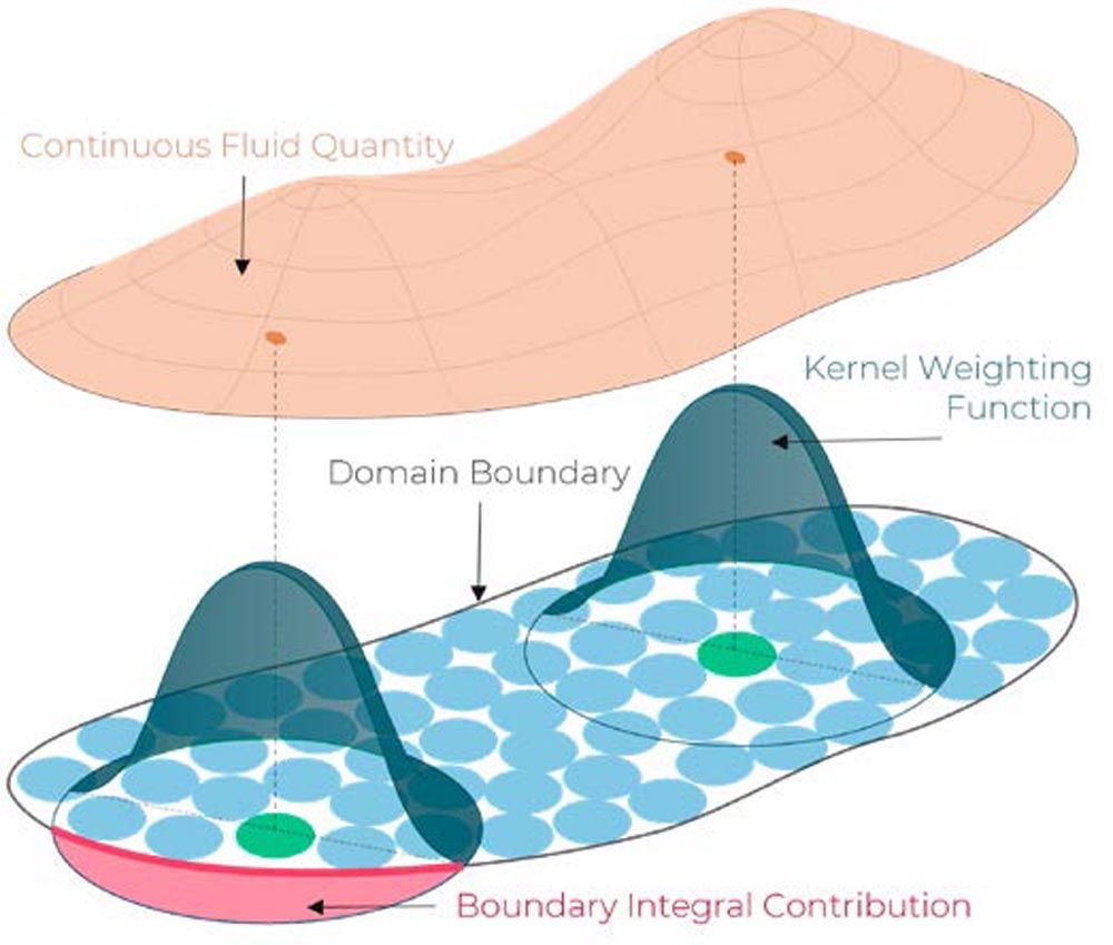
Figure 1—3D visualization of the SPH interpolation within the fluid (right) and with domain boundary contribution (left).

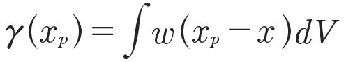
A weighted interpolation, i.e., the kernel function w, at these points, is used to determine its properties based on its distance from adjacent particles and their physical quantities 𝛾. As the interpolation radius may extend beyond the presence of fluid, e.g., at walls, a renormalization factor 𝛾 is introduced to account for the missing content and ensure at least zeroth order consistency (Ref. 30). The described interpolation reads:

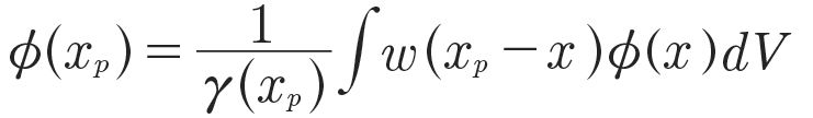
(3)

Here, the Wendland kernel of the fifth order is used as a weighting function. Using the derivative of the kernel, the SPH formalism allows for an approximation of spatial derivatives, which is crucial for solving partial differential equations numerically. The concept is illustrated in Figure 1. Specific care has to be taken for the consideration of boundary handling. Consider the lower green particle at position x_p then, with its kernel function w, the kernel interpolation of a derivative for arbitrary quantity 𝛾 will have a volume integral contribution (∫ … dV)and a boundary integral contribution (∫… dB). The first comes from within the fluid, i.e., the contribution from the surrounding particles and the latter stems from the kernel overlapping with the wall. Here n is the inward-pointing surface normal. To ease readability, the renormalization term is ignored. Integration by parts yields (Ref. 31):

(4)

Navier Stokes Equations in a Weakly Compressible Formulatio

Liquids are considered incompressible if the density remains constant. This is true for fluid speeds significantly below the material’s speed of sound or if pressures are not extreme. In the current work, a weakly compressible modeling approach is utilized allowing for small density changes, i.e., less than one percent. An equation of state links the pressure directly to the density change.

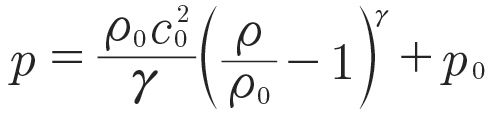
The mathematical basis of fluid dynamics is derived using this preposition. Incompressibility is considered for the derivation of the momentum equation. Contrarily, the continuity equation is solved in its compressible form to account for the change in the density. Here, the equation of state proposed by Cole (Ref. 32, 33) is used. This yields the governing equations for weakly compressible SPH in the Lagrangian formulation:

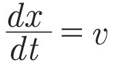
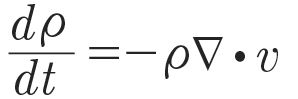
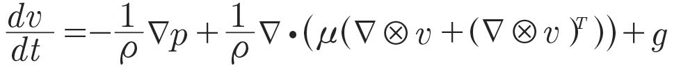
(5)

with the position of the particles x, velocity v, time t, density 𝜌, pressure p, dynamic viscosity 𝜇, gravity g, background pressure p₀, artificial speed of sound c₀, reference density 𝜇₀ and exponent 𝛾, which is chosen as 7.0 for liquids like oil (Ref. 33) and 1.4 for gases like air (Refs. 34, 35). It should be noted that the artificial speed of sound is a numerical trick to enlarge the time step, i.e., fast computation times, while receiving physically sound results.

Equation 5 is discretized using the SPH formalism. The temporal derivates are discretized using a modified Runge-Kutta 4 (Ref. 37) scheme, separating the acoustic and advective time steps to allow for faster computation (Ref. 38). To improve numerical stability and the quality of the pressure field, an additional diffusive term is added to the continuity equation (Ref. 39). To ensure a regular particle distribution while avoiding unintended particle clumping, a particle shifting technique is applied (Ref. 40). This improves the interpolation quality of the scheme (Ref. 41) while maintaining the overall volume of simulated fluid. The utilized method is inspired by Ref. 42 and 43. In this work, no turbulence model is utilized.

Wall Boundary Conditions

For the wall boundary conditions, there are two major approaches to representation:

• The boundaries are thickened with so-called dummy particles, that can be included in the regular particle interaction (Ref. 32).
• Integral boundary conditions use a segment-based mesh representation of shapes (Ref. 44).

In Sabrowski et al. (Ref. 35], the different boundary condition approaches are discussed specifically for gearbox applications. This work uses a segment-based mesh representation to treat boundary conditions. This approach was chosen as it allows for a very accurate and native representation of computer-aided design (CAD) geometries in the SPH method and ensures to account for the boundary contribution of the SPH interpolation.

Particle Refinement Techniques

One of the five grand challenges of SPH is adaptivity (Ref. 45), which is generally the usage of multiple particle sizes within one simulation. The ideal particle-based solver adapts the particle size so that the numerical resolution is fine enough in areas of interest to resolve desired flow phenomena while being computationally fast and without introducing numerical errors. Having particles of different sizes interact in a naïve manner with one-another does immediately violate the conditions, such as:

• Larger particles would have larger kernel sizes, thus, considering smaller particles for the interpolation that do not see the larger particles. This would violate Newton’s third law, i.e., reaction would not equal action,
• Compensating for this caveat by enlarging the kernel radii for smaller particles would lead to a significantly increase in particle neighbor count, thus, computational performance would decrease.

Multiple ideas exist like an adaptive particle splitting technique into multiples of their previous size based on certain pre-defined flow conditions. Similarly, these particles are merged, or de-refined. If the algorithm avoids the issues mentioned above, one idea can be to merge particles of versatile sizes as pairs or small groups. As pointed out by Chiron et al. (Ref. 46), this process can become computationally costly and faces difficulties when the coalescence rate differs from the refinement rate since particles may be merged as pairs but created as eightfold, twenty-sevenfold etc. An additional challenge is introduced as the de-refining step has been shown to react sensitively to non-regular fields (Ref. 45).

Another idea consists of small layers that coexist on top of the coarse domain to avoid overlapping of the kernels (Ref. 35). Here, the large, further denoted as coarse, particles enter the region of interest and, in the buffer layer of the fine particles, are split into finer particles. Fluid properties are interpolated into this layer by SPH formalism from active to passive particles ensuring information coupling of fine and coarse regions. Afterwards, the flow equations are solved on the fine particles and coarse particles are passively advected. Once the fine particles leave the buffer zone, the flow equations are solved by the re-activated coarse particles and the fine ones are deleted. This ensures mass conservation for the coarse layer. The process is schematically shown in Figure 2 and will be used in this paper.

Figure 2—Particle refinement method with the multi-layer approach in 2D. Coarse particles are split into four fine particles in a buffer zone. The fine particles are active in the refinement zone.

Hydraulic Loss Evaluation Method

The calculation of churning losses is executed using pressure F_pi and viscous forces F_vi acting on the i-th rotating boundary triangle with area A_i and normal vector n_i as:

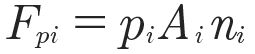
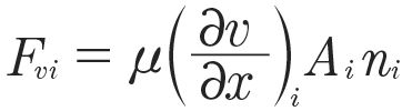
(6)

The specific torque around the rotational axis of each component j can be calculated as:

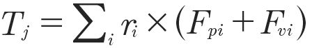
(7)

with the lever r_i. However, a more general approach is exploited to calculate the local power P_i by its definition as force F acting on a segment scalar product with the segment velocity v_i:

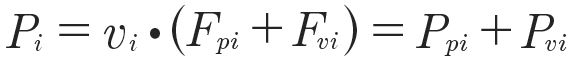
(8)

Integrating over the whole component leads to the corresponding overall power losses by means of viscous P_vi and pressure P_pi:

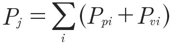
(9)

which will be used to evaluate the power loss distribution for each component. Equation 8 circumvents the necessity to individually account for the torque of one roller bearing rotating around its axis and the axis of the shaft. This formulation is universally applicable.

Tapered Roller Bearing Kinematics

The kinematics calculation of the gears is done by applying an ideal gearing ratio and requires no further explanation. The bearing’s motion is assumed to be slip and deformation free, thus, modelled by ideal kinematic slip conditions at the contacting surfaces. The equations must be derived in the form of two motions:

• The rigid rotation of the cage and rollers around the axis of the inner ring—𝜔_cage
• The rotation of each roller around its axis which is moved by the cage’s motion—𝜔_roller

Since the motion of an axial, ball and cylindrical bearing represents a special case for a bearing with a roller that moves with tilted roller axes, a general set of motions is derived based on Figure 3.

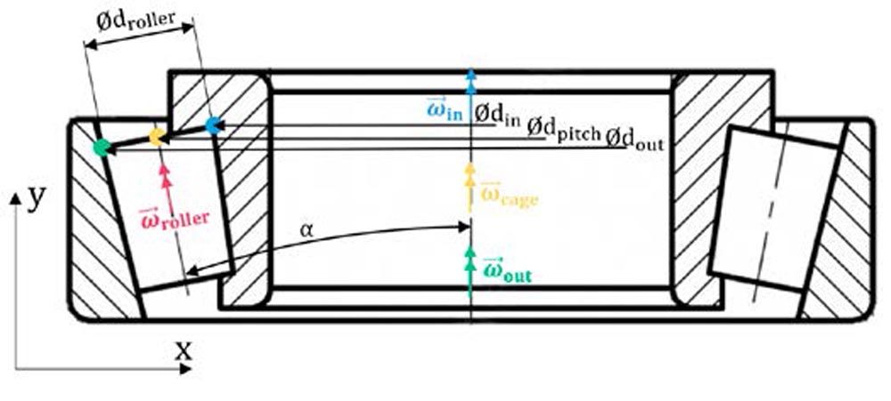
Figure 3—Schematic tapered roller bearing kinematic description.

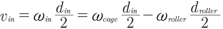
The bearing moves slip free around the inner and outer race, thus, any set of points for a representative roller diameter suffices to derive the kinematic relationship. Without loss of generality, consider the three marked points (•,•,•). At the outer race (•), the circumferential velocity of the outer race must equal the superposition of the roller velocity added to the cage velocity. At the inner race (•), the circumferential velocity of the inner race must equal the superposition of the roller velocity subtracted from the cage velocity. Velocities are written in terms of rotational speed and effective diameter that yield:

•

(10)

•

(11)

Substituting d_in = d_pitch-cos 𝛼 d_roller and d_out = d_pitch+cos 𝛼 d_roller with 𝛼 being the angle between the inner race axis and roller axis eventually leads to:

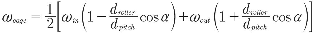
(12)

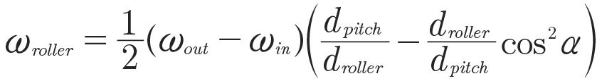
(13)

Experimental Setup

The torque test bench Kegelradprüfstand (KRPS) at Dresden University of Technology (TUD) is used for this study. It consists of two slave and two test gearboxes of similar characteristics shown in Figure 4. Test gearbox 2 is investigated in detail. The load torque is applied on the pinion side, torque is measured with an HBM torque transducer of type T40B on the shaft of the pinion and as well as the wheel.

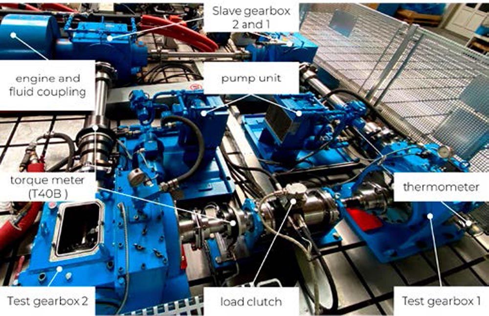
Figure 4—Bevel gear torque test bench (KRPS) at Dresden University of Technology.

The temperature was measured at the bottom of the oil reservoir. A temperature of 60 ± 2°C was ensured throughout all torque experiments. For the experiments, the oil Mobilube HD 80W-90 was used. The oil properties at the respective investigation temperatures are given in Table 1.

The test gearbox comprises a bevel gear stage with a gear ratio of 3.08. The pinion shaft is supported by two roller tapered bearings in the X-mounting position, the wheel is supported by two smaller tapered bearings in the O-mounting position and an additional cylindrical roller bearing. The digital model (Figure 5) does not include an active lubrication system in between the pinion bearings and the meshing zone as well as the pumping system and pipes at the bottom of the reservoir. This system cannot be removed nor switched off. Previous studies at the test rig have shown that the lubrication effect of the injection system is negligible. It is not clear if this holds for power losses as well. The uncertainty consequences are discussed at a later occasion.

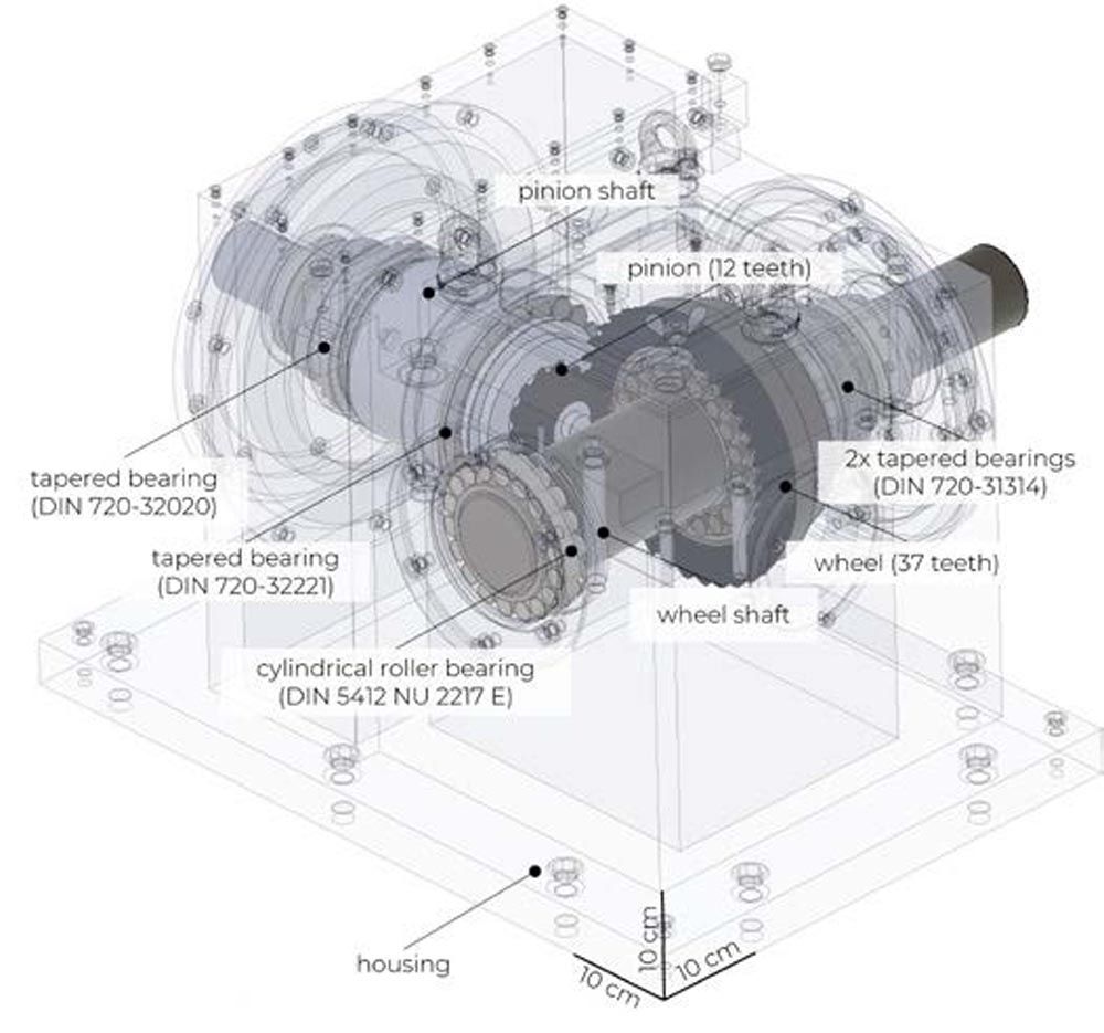
Figure 5—Geometry model of the test gearbox. Neither injection nor pumping system are included.

The average torque loss was measured for rotational speeds from 1,200 to 1,800 rpm, filling heights of 10, 45, and 85 mm below the centerlines and both turning directions. The gearbox of dimension 700 x 500 x 500 mm contains around 16 L oil at the highest filling level. The rotational speed was increased stepwise; this increase was followed by a stepwise decreasing measurement resulting in two torque readings that cover 15 seconds of measurement time each. The load-dependent, injection-induced and sealing losses were subtracted by employing one minimum lubricated test run for both turning direction. The introduced uncertainty is discussed at a later occasion. The gears are engaged in driving mode for all operating conditions. For all tests, a constant load of 1 kNm had to be applied on the pinion side to avoid damage to the slave gearboxes due to gear hammering. The following tests have been conducted for both turning directions, which is inwards (IN) if oil is immediately dragged into the meshing zone and outwards (OUT) otherwise. The gear characteristics are given in Table 2.

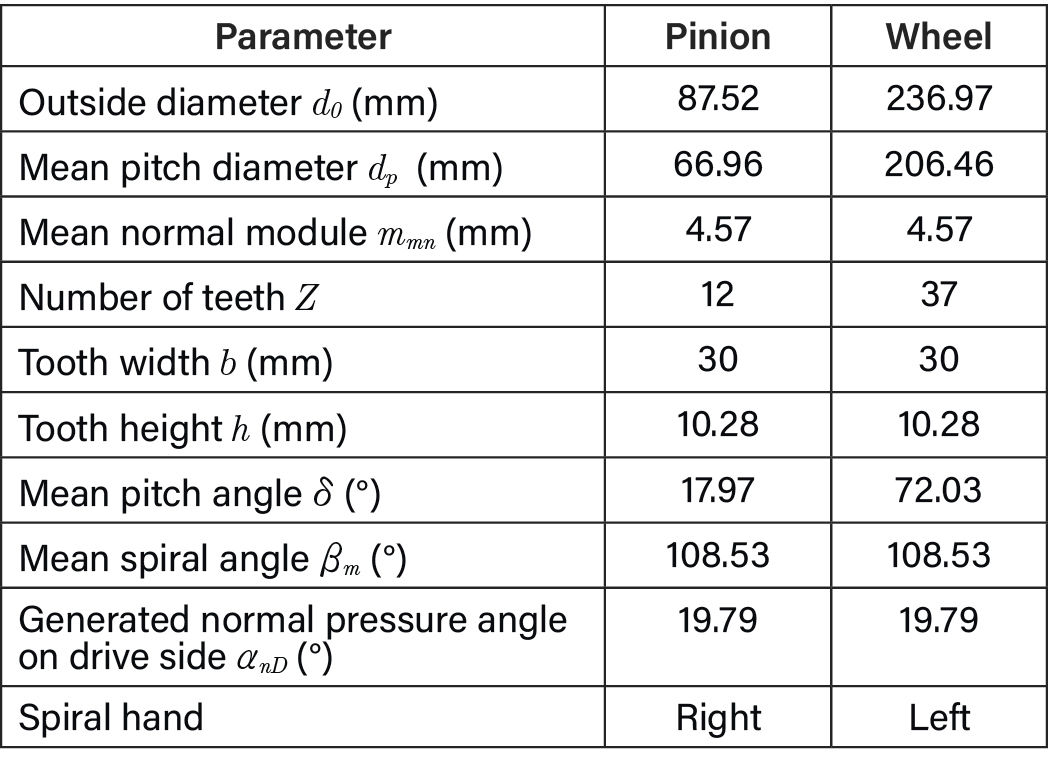
Table 2—Bevel gear pair characteristics.

Numerical Setup

For a visual comparison, the cold start situation (26°C and 600 rpm) was captured by removing the top lid of the housing. The amount of aeration has been visually verified to be small after the test run. Visual validation of the oil distribution has been conducted by Ref. 36. For the following section, bearing DIN 720-32221 is addressed as the larger pinion bearing 1 (P1), bearing DIN 720-32020 is addressed as pinion bearing 2 (P2), bearing DIN 5412 NU 2217 E as wheel bearing 1 and both bearings DIN 720-31314 together as wheel bearing 2 and 3. Only the last two are provided with a cage geometry.

The simulations are executed as follows: Spatial particle refinement zones are located around the gears, bearings and the pinion’s shaft between the supporting bearings as visualized in Figure 6.

Figure 6—Initial discretization and geometry setup for nominal filling height of -10 mm below gear axes. Dark blue areas represent coarse particles (1.4 mm), light blue refined particles (0.7 mm). Transparent blue shapes indicate the refinement zones.

Both gears, shafts, and contacting roller bearings with cages linearly accelerate to full speed at 0.1 seconds and hold the terminal velocity for 0.4 seconds. The ramp-up is chosen to allow for faster quasi-stationary convergence. Starting with the terminal velocity introduces a shock similar to a splashing event into the simulation system whose effects take longer to decay. The movements of the bearings and cages follow the ideal kinematic contacting conditions. The simulation finishes at 0.5 seconds. The churning loss results are averaged over the last rotation of the wheel. The simulated hydraulic loss signal over time for a full system rotation of 1,600 rpm for the outward turning direction is shown in Figure 7. All simulations were conducted in parallel on the cloud-native simulation platform Dive Solutions on CPU AMD EPYC 7V73X within 29- and 40-hour simulation time with the solver Dive SPH 3.4.1 with varying particle counts of 7 to 8.5 million.

The study Ref. 36 investigated the gear interaction space without bearings and found negligible loss differences for spatial resolutions smaller than 1.5 mm. To allow for a numerical discretization through the pinion and wheel shrouding gaps, a minimum global particle size of 1.4 mm must be chosen, which fulfils the particle size requirements of the study mentioned above. However, the previous study did not investigate the resolution sensitivity of hydraulic losses for the bearings or the shafts. Compared to the data presented in the study (Ref. 36) and this study the following differences are present:

• Postprocessing routine:
  • The newly utilized postprocessor reconstructs the exact forces present on the walls to accelerate the fluid.
  • The old, utilized postprocessor extrapolated the fluid-induced forces of interest from the fluid data onto the walls.
• Solver modelling:
  • A new particle-shifting technique has been used in this study.
• Spatial discretization:
  • Full system simulations were done with a 1 mm particle size in the previous study.

The consequences of these changes are manifold and cannot be summarized with a clear trend.

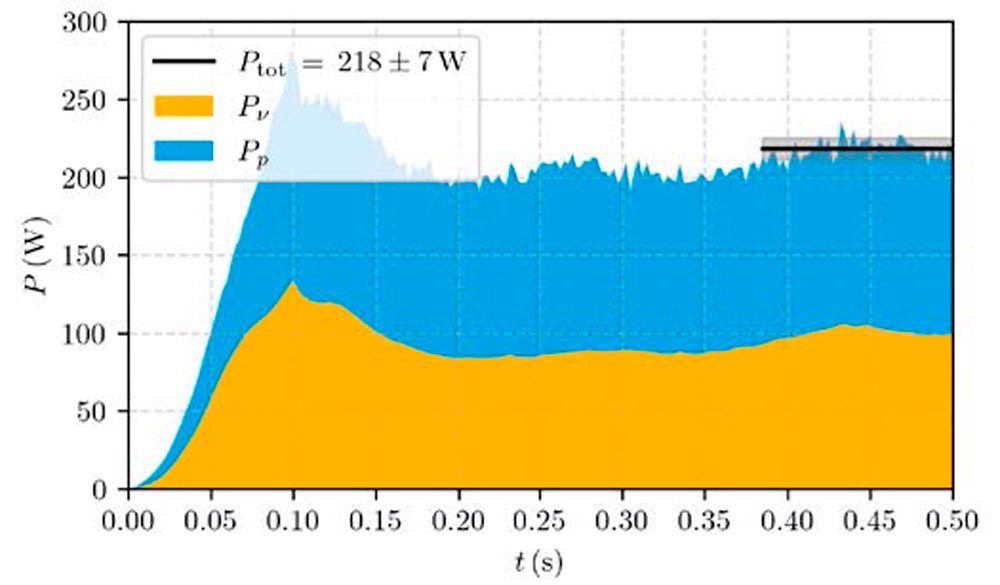
Figure 7—Viscous P_v (yellow) and pressure P_p (blue) induced hydraulic losses for the full system’s OUT case without bearing subsystems at 1,600 rpm. Overall hydraulic losses are averaged over one full rotation of the wheel.

The study Ref. 36 pointed out that the churning loss contribution from the tapered roller bearings in the pinion becomes substantial and needs to be captured. To keep the simulation effort low, the following method was employed: Based on the fluid distribution at the last output, the flow field around each bearing’s proximity is extracted and further refined. This subsystem is investigated in a separate simulation until the results reach a stable value. The process is elucidated in Figure 8, where the fluid distribution’s contour around the large roller bearing of the pinion is extracted and yields as a fluid filling for a subsystem simulation. To ensure mass conservation between the old and new system, the fluid contour is slightly thickened. The validity of this process is based on the assumption that a) the influence of the subsystem’s axial boundaries is negligible and b) the loss signal becomes quasi-stationary before a significant amount of flow is moved axially through the bearing. Fixing the particle size globally at 0.25 mm for all bearing simulations lead to optimized runtimes of 0.5–4 hour per subsystem simulation for setups with 2 to 14 million particles allowing to complete all simulations within two days.

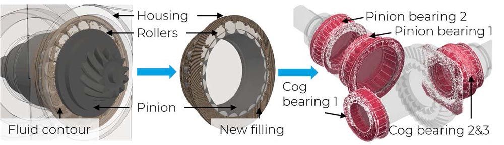
Figure 8—Visualization of the subsystem derivation step from a full system simulation (left) to a detailed system simulation of pinion bearing 1 (center) to all four subsystems (right).

Starting the subsystems simulation from the derived fluid distribution at terminal speed induces a shock at the beginning of the simulation that quickly decays as shown in Figure 9 for the pinion’s bearing 1 in the OUT case at 1,200 rpm. The pressure loss signal quickly starts to oscillate after the rollers covered one-sixth of the pinion shaft circumference at 12 milliseconds.

A side note on the observed oscillation frequency: it is fixed at around 120 Hz for this subsystem simulation. It does not seem to be related to the roller rotational speed around their axes (65 Hz) the roller frequency around the pinion (8.5 Hz), or the pinion’s rotational speed (20 Hz). Similar effects were observed for the other bearing subsystems at 1,200 rpm and 1,600 rpm but not for 1,800 rpm at the given output frequency. The amplitude of this oscillation is relatively lower for the wheel’s bearings compared to the pinion’s bearings and is only visible at higher speeds. Lowering the oil level increases the amplitudes at a given rpm. The analysis of their origin is left for further research.

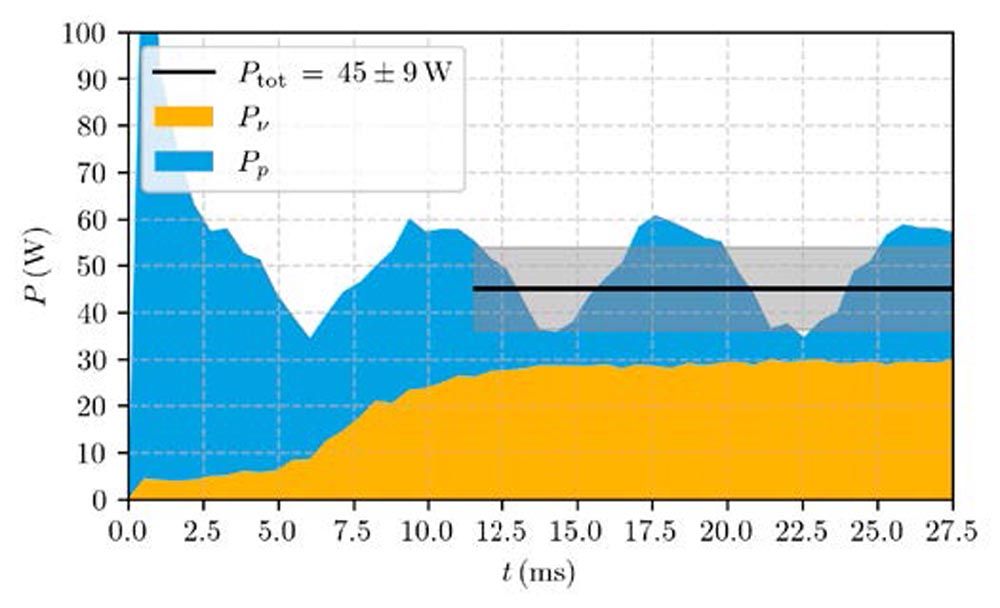
Figure 9—Viscous P_v (yellow) and pressure P_p (blue) induced hydraulic losses for rollers in the subsystem of pinion bearing 1 in the OUT case at 1,200 rpm. Overall hydraulic losses are averaged over 60 percent of the simulation length.

All consecutively shown data are combined results of the full system’s pinion and wheel hydraulic losses and bearing subsystem analyses if not stated otherwise.

Results

Bearing Investigation

Modelling the ideal kinematics of bearings becomes challenging for grid-based methods to avoid degeneration of mesh cells and, thus, time convergence challenges. Even particle-based methods have lower geometry quality demands, so they are simulated with a simplified motion i.e., as a solid body rotating with the average of the relative rotational speed difference between the input and output shaft. The difference in terms of wetting and loss distribution of both approaches are investigated on the example of the pinions’ bearings 1. To avoid the influence of surrounding geometries, both simulations were executed as a subsystem simulation from the fluid field of the 1,600 rpm-OUT case.

Time-averaged data is summarized in Table 3. Despite being less wetted, the ideal kinematics come with 67 percent higher hydraulic losses than the case with simplified kinematics. The reason for this difference is found in the negligible share of viscous losses for rollers under these kinematic conditions.

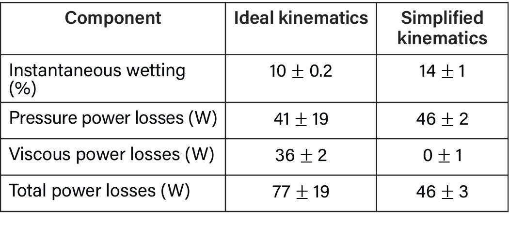
Table 3—Instantaneous wetting and hydraulic power loss share comparison of pinion bearing 1 subsystem simulation at 1,600 rpm in the OUT case for ideal and simplified kinematics.

Considering the surface wetting distribution, pressure, and viscous hydraulic losses, in Figure 10, the shaded contours in the left column indicate a more wetted at the contacting zone at the outer race than on the inner race for both cases due to the general pumping behavior of a tapered roller bearing. The exact roller motion transports oil from the outer to the inner race and reduces the oil distribution shift. In contrast, the shift is more prominent for the simplified motion implying less oil on the inner race than on the outer race. Still, pressure-induced losses are of similar magnitude for the simplified motion despite having more oil at the outer race and a numerically higher velocity. For the ideal rolling motion a higher pressure is being built up by dragging the fluid on the surface into the contacting zone which counteracts the motion overall motion of all rollers. Since velocity equilibrium is enforced on the inner race, the same effect happens there but the pressure force acts beneficially in the direction of the overall roller’s motion. In the simplified case, less fluid reaches the contacting area at the inner race. Combining this fact with lower speed leads to lower simulated pressured-induced losses.

While pressure-induced forces stem from a normal force counteracting the motion of the body, viscous-induced forces stem from forces acting tangentially against the direction of motion of the body. Keeping this in mind, fluid shear rates must be large in the contacting areas when the flow is dragged from the area of high volume into the area of low volume, thus, must escape elsewise. However, power losses are only produced in areas of high velocity due to the definition of power times velocity. At the outer race, the low velocity magnitude renders viscous induced power loss small but makes them substantially larger at the inner race for the correct bearing motion. For the simplified kinematics, the squeezing effect into the contacting zone is not captured, thus, viscous losses are negligible in case. At the inner race, the small amount of oil that reaches the contacting zone creates large friction on the shaft as this has a larger circumferential speed than the rollers.

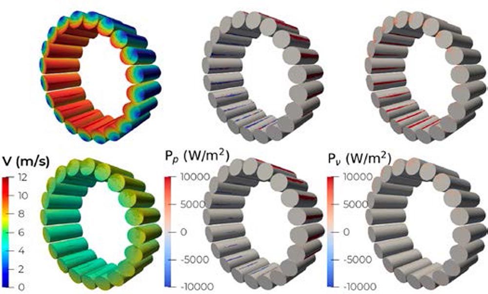
Figure 10—Comparison of the exact bearing kinematics (top) and a rigid rotation with half the shaft’s velocity (bottom) in the subsystem simulation of pinion bearing 1 at 1,600 rpm, OUT, for velocity (left) with wetting- (shaded), pressure- (center) and viscous- (right) induced losses.

An overview of viscous and pressured-induced loss changes from the full to the subsystem analysis is given in Figure 11 with the two largest bearing contributions, pinion bearing 1 (P1) and pinion bearing 2 (P2) and the loss change from the full system to the subsystem simulation. The change from 0.7 mm particle size resolution to 0.25 mm particle size becomes more prominent for larger rotational speeds indicating that larger speeds come with both higher velocity and pressure gradients. For an under-resolved simulation, i.e., velocity gradients are not captured at all, halving the particle size would lead to doubling the viscous loss share due to better resolution of the boundary layer. Here, the largest difference (1,800 rpm, OUT case, P1) is 2.5, which is lower than the particle size ratio of 2.8. Additionally, the wetting increased from 9 to 10 percent. Thus, boundary layers are partially resolved. The change in pressure can go both ways: for lower rpm, the pressure share on total losses reduces from coarse to fine resolution as particles are less as less geometrical squeezing appears. At higher rpm, resolving the physical squeezing in more detail reproduces the correct pressure gradients. Thus, ensuring convergence for both loss shares is paramount to determining convergence. More critically, under-resolving can lead to wrong trends as seen for the pinion bearing 2 trends from 1,600 to 1,800 rpm. The pressure share was not resolved at all. Thus 0.7 mm particle size is not sufficient to resolve pressure gradients in between the smaller rollers. Increasing the resolution did capture some pressure gradients and increased wetting by about five percent. A finer resolution is advised for future studies.

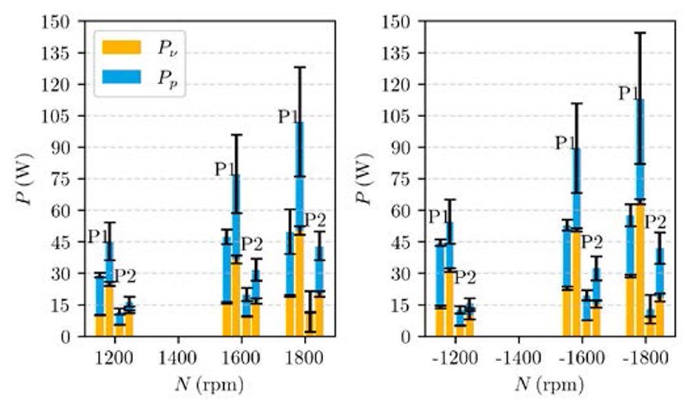
Figure 11—Viscous P_v (yellow) and pressure P_p (blue) induced churning losses by pinion bearing 1 (P1) and pinion bearing 2 (P2) in coarse (0.7 mm, left) and refined (0.25 mm, right) resolution over rpm. OUT (left chart) and IN (right chart) case are shown.

The subsystem simulation reveals that pinion bearing 2 is virtually unaffected by the turning direction. The measured amount of oil within the bearing is equal for all subsystems. Contrary, pinion bearing 1 churning losses are constantly more than 10 percent larger for the IN direction, more specifically, due to more than 15 percent larger viscous losses. This correlates with a more wetted area for the inward direction for all speeds for the direction of the inward as listed in Table 4. It is noticeable that a relative increase in wetting leads to a lower relative increase in viscous churning losses. Since the high viscous power loss zone—contacting zone of the roller at the inner race—is already filled, the additional wetted area is in regions of lower velocity gradients. A detailed investigation of the loss mechanism is given in the next investigation.

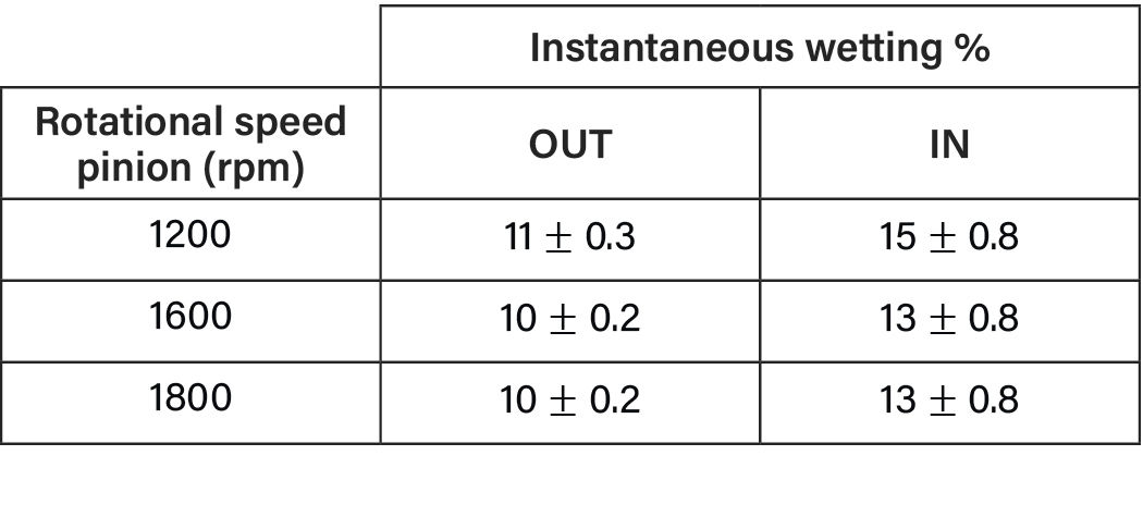
Table 4—Instantaneous wetting of pinion bearing 1 over rpm and turning direction.

Influence of Turning Direction

Turning direction is considered to have a substantial impact on hydraulic gearing losses. This effect is commonly known to be related to oil squeezing for high oil levels, specifically if an oversupply of oil is dragged into the gear meshing zone as could be expected for the IN case.

The simulations of both turning directions at 1,600 rpm input speed capture this trend as well—overall hydraulic losses are over 20 percent larger when oil is dragged into the meshing zone compared to out of the meshing zone. The same ratio was found in the experimental investigation. From Table 5, it is deducted that wheel bearing 2 and 3 as well as pinion bearing 2 are located away from the gear interaction zone, thus, losses are virtually unaffected by a change in turning direction. Although located in the gear interaction region, the cylindrical roller bearing on the wheel does not show a change in churning losses. Thus, the dynamic oil level change in the proximity of this bearing is not affected by the turning direction in this speed range. All components mentioned above are rotationally symmetric. Only asymmetrical flow towards the bearings due to asymmetrical geometrical changes close to these regions can cause noticeable differences in churning losses. Since pinion bearing 1, pinion and wheel interact with the fluid nearby, all differences are found for those three components. More specifically, all three components have larger losses in the IN case, with a 10 percent increase for the wheel, a 15 percent increase for the pinion bearing 1 and a 43 percent increase for the pinion.

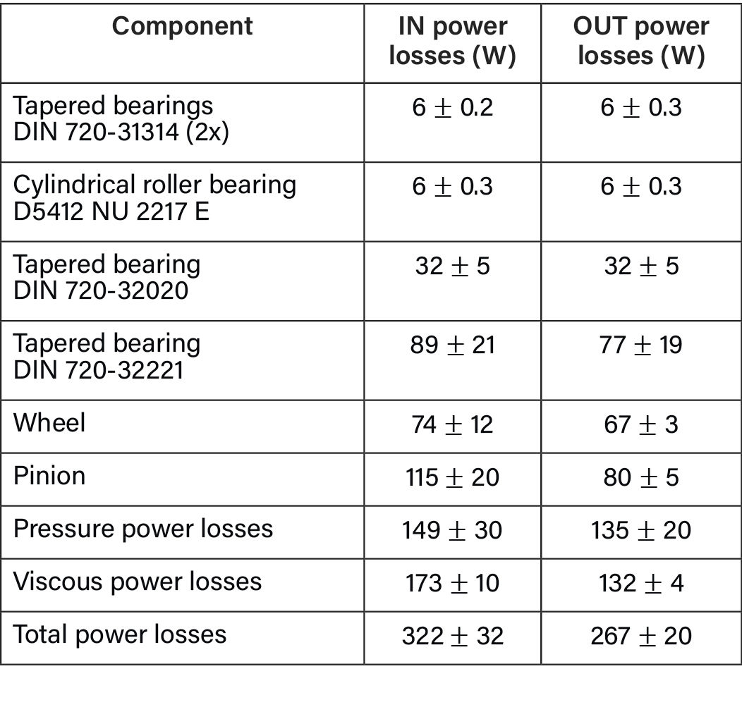
Table 5—Component-wise load-independent power losses for the IN and OUT case at 1600 rpm pinion rotational speed.

The surface churning loss distributions for the gears are displayed in Figure 12. The wheel’s loss contribution in the submerged section is more present for the OUT case than the IN case due to the beneficial teeth shape that guides oil with the wheel’s motion. This oil is quickly thrown off the wheel towards the housing and a smaller share of the airborne oil falls or impinges at the housing close to the engagement zone. For the pinion, the same mechanisms apply with even less oil being guided back to the engagement zone due to the box-shaped housing.

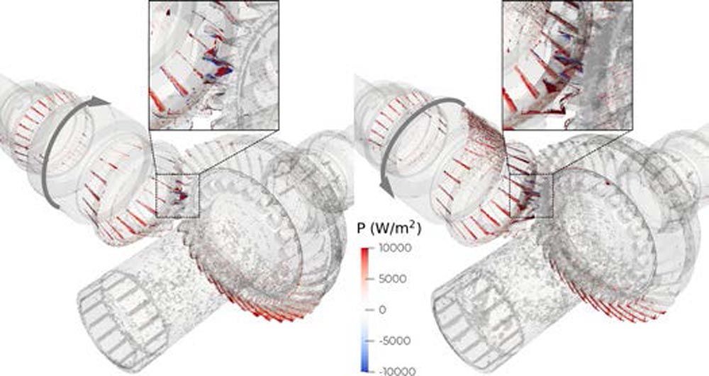
Figure 12—Churning loss distribution over the gears for 1,600 rpm at the input shaft in the OUT case (left) and IN case (right). Instantaneous wetting is indicated as shaded area. Zoom on the meshing zone on top.

On the contrary, the IN-case oil is piled up in the engagement zone due to the wheel pushing a substantial amount into this corner of the box (i, Figure 13). The difference in both clips represents over 75 percent more mass for the inward case in the region of interest. This excess oil is squeezed out of the engagement zone with the spin direction of the wheel into the pinion bearing 1. This explains why more oil reaches pinion bearing 1 in the IN direction than the OUT direction. Effectively, this effect also prevents oil from in between the pinion bearings to be pumped out leading to larger viscous losses around the large pinion shoulder (right, Figure 12). This effect comes also with larger viscous losses at the inner race, being part of the pinion (zoom, right, Figure 12). The oil is pumped out of the bearing at larger rotational angles (ii, Figure 13). Lastly, most of the oil is picked up again by the wheel and pushed to the opposite side of the housing (iii, Figure 13).

For the OUT case, oil that spun off the wheel, partially dripped back from the housing on the wheel and dragged into the engagement zone (1, Figure 13). There, it is axially squeezed towards the wheel shaft (3, Figure 13) leading to lower hydraulic losses due to the squeezing in this turning direction. As there is no large-scale flow created by the gears into the pinion bearing 1, less oil is pumped out of the bearing (2, Figure 13).

The main source—more than 50 percent of the increase—for additional losses in the direction of the inward stems from the pinion that a) has additional pressure contributions due to pushing more oil with the tooth flanks and b) larger viscous contributions due to more wetted area in between the pinion bearings and on the inner race of pinion 1.

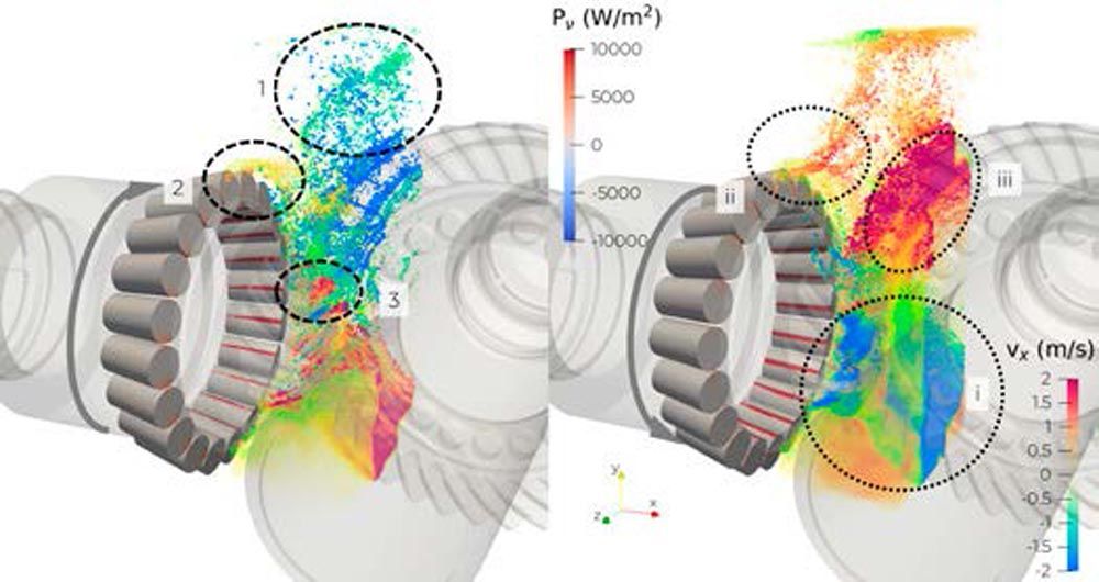
Figure 13—Clip of the axial velocity distribution in the gear engagement zone for 1,600 rpm at the input shaft in the OUT case (left) and IN case (right) with highlighted hydraulic loss mechanisms and viscous-loss distribution of pinion bearing 1.

The difference measurement for the experiment gave 510 W for the OUT and 610 W for the IN case as hydraulic losses of the system. Thus, the relative increase of 20 percent from outward to inward direction is replicated, however, the quantitative agreement is at 52 and 54 percent for the OUT and IN cases respectively.

Influence of Filling Height

Lowering the filling height is undoubtedly a simple measure to lower the hydraulic losses since gears are less submerged in oil. Table 6 summarizes the outcomes for an oil level immediately underneath the pinions’ teeth. Simulated churning losses dropped by 27 percent, mainly due to a decrease in viscous loss contribution. Specifically, pinion churning losses plummet to 47 or 53 percent for the OUT and IN cases respectively. Considering the loss mechanism discovered in the previous section, those will be less present in cases where a) the pinion does not submerge in oil and b) fewer wheel teeth are immersed in the oil so less oil is dragged out from the reservoir. The splash pattern is still similar to the nominal filling height except for a lower oil column next to the engagement zone for the IN case at a lower oil level (Figure 15).

The simulation detects no change in hydraulic losses for the pinion bearing 2 in the subsystem simulation. Indeed, although the simulated masses for the pinion bearing 2 subsystems are 27 percent lower for the lowered level, the losses of the rollers show no change. The origin of this outcome is not clear as the rollers are indeed better wetted for the nominal filling height than for the lowered filling height, which is mainly found to be true for the front and back faces. As the main loss mechanism in the rollers was found to stem from the contacting region, the explanation might be that the pickup volume between the rollers is limited for a defined operating condition and not noticeably affected by filling height. Further research is required to understand this behavior.

Again, simulated losses are lower than the experimentally determined ones. With 270 W for the OUT and 370 W for the IN case difference measurements, experimental losses are met by 72 and 63 percent in the simulations of the OUT and IN case respectively.

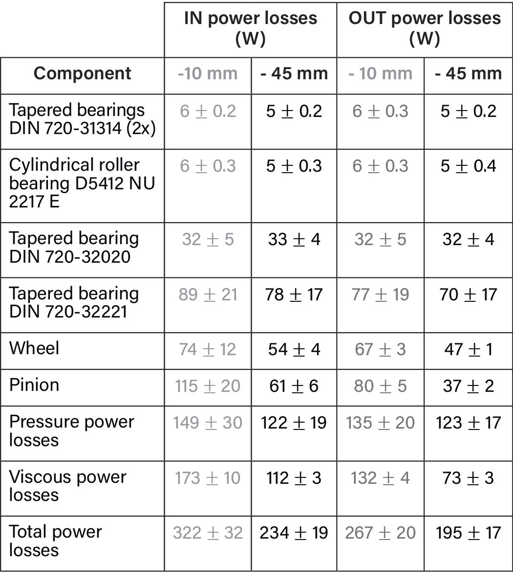
Table 6—Component-wise hydraulic power losses for the IN and OUT case at 1,600 rpm for the lowered oil level in comparison with the nominal filling height.

Influence of Rotational Speed

An overview of simulated losses over pinion rpm is given in Figure 14. Simulated losses increase with rotational speed. If 1,200 and 1,600 rpm results are considered, the simulated losses for 1,800 rpm exceed the linear extrapolation between both points indicating an over-proportional growth of churning losses with rpm with a maximum deviation of 7.5 percent. Still, for the simulated range, a linear trend is an acceptable simplification. If this trend is assumed, the linear least square regression yields a slope of (0.404 ± 0.006) W/rpm for the IN and (0.310 ± 0.032) W/rpm for the OUT direction. This observation is also valid for an artificial regression point of 0 W at 0 rpm. Therefore, simulated IN losses are not only larger than those in the OUT case but also grow 30 percent faster with rpm.

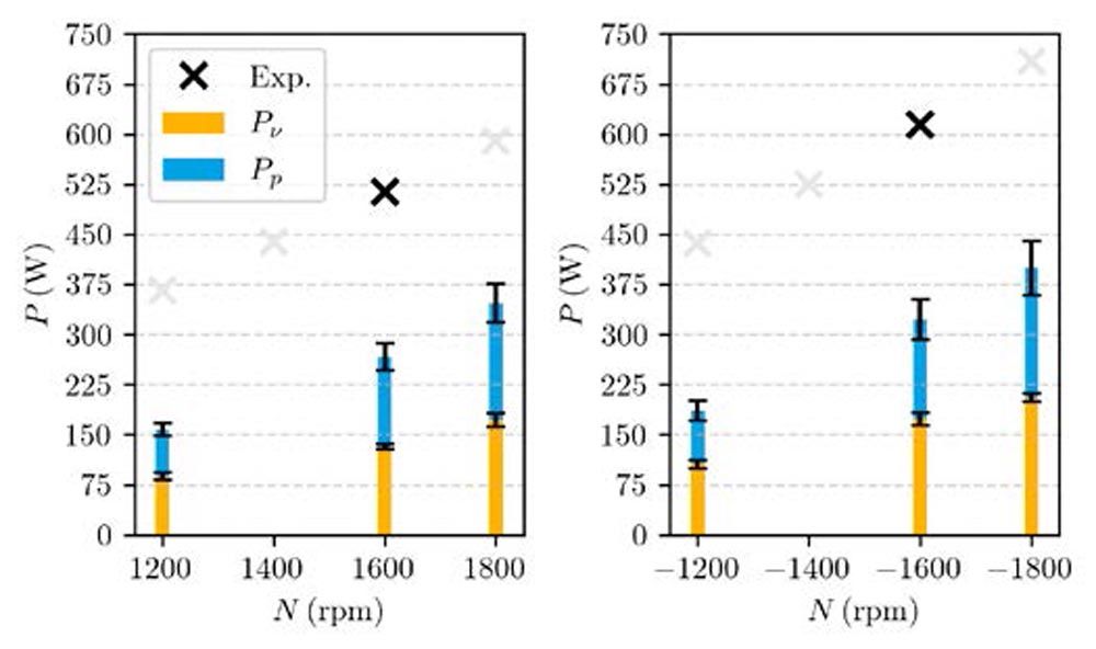
Figure 14—Viscous P_v (yellow) and pressure P_p (blue) simulated churning losses compared to experimental data (×) over rpm. OUT (left chart) and IN (right chart) case are shown. Bright marker indicate linearly extrapolated losses.

Part of this faster growth is likely to be seen in the wetting distribution and indicated surface flow direction Figure 15. While the wheel-induced splash pattern at the housing side opposing the pinion becomes more prominent for the OUT direction (-10 mm, left), this effect does not drive more oil towards the engagement zone of the gears (-10 mm, right). For the IN case, more is dragged upwards and against the housing in proximity to the gear meshing zone, which is a leading factor of churning losses (-10 mm, right).

The individual loss contributions show a different growth trend. Both contributions grow in absolute value with rpm, but pressure losses grow faster than viscous losses. As described in Ref. 36, pressure losses come with a higher order dependency on rotational speed, which is observed in this case as well.

The experimental trend is deducted from trends and not by measurements, thus, results with light grey crosses must be considered as estimates. For 1,600 rpm in both turning directions, load-dependent and load-independent losses were measured and losses with the same load but without any oil were deducted. The remaining difference accounts for hydraulic losses. As total losses followed a clear linear trend between 1,200 and 1,800 rpm for both directions, the measured delta has been scaled with rpm and deducted for all other operating conditions. This approach must yield a linear trend in hydraulic losses. Therefore, there is no additional value in comparing results for 1,200 and 1,800 rpm between simulation and measurement since results must be similar to the ones at 1,600 rpm.

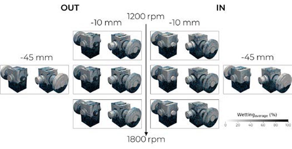
Figure 15—Average wetting on housing surface for OUT (left) and IN (right) case over pinion rotational speed and filling height. Flow paths are indicated with surface glyphs.

Experimental and Numerical Uncertainty Discussion

The difference in power losses from the filled and drained gearbox is considered to give hydraulic power losses. The results at the KRPS resulted in 610 W for the IN direction and 510 W for the outwards turning direction at 1,600 rpm pinion speed filling height 10 mm below the gear axes. The differences between the experiment to the simulation can be clustered as follows:

• Bearing representation:
  • Pinion bearings and the cylindrical roller bearing on the wheel come with cages which were not present in the CAD data.
• Measurement techniques:
  • Tapered roller bearings must be applied with pre-load, which results in loss contribution for both, load-dependent as well as load-independent classification.
  • The drained IN direction was investigated after the drained OUT direction was measured
  • Gear-load for 1 kNm to avoid gear hammering required a torque measurement device with high uncertainty for the differentially determined hydraulic loss range
• Active lubrication:
  • The test rig contains an active lubrication system injecting from above into the meshing zone and in between the pinion bearings. Neither is geometry present nor is the volume flow known.
  • This system cannot be shut down even with drained reservoirs.
• Oil properties:
  • Oil data was taken from the data sheet and not measured.
  • Oil reservoir temperature was considered as the overall oil temperature

For the simulation, the largest uncertainty is found to be the loss results in terms of particle size.

Starting with the bearings, including the cage is likely to increase viscous losses due to more area shearing the oil and squeezing in between the cage and rollers. It can be assumed that the cage can create an additional flow resistance leaving more oil in the zone between both pinion bearings. The effect is further increased by considering the active lubrication between the pinion bearings.

The assumption of oil properties could lead to changes in both directions. It can be assumed that this effect is of lower order both, oil properties of different charges and age as well as local temperature variation should not affect viscosity and density by significant factors.

Similarly, changes in pre-load with rotational speed or dynamic motion of the bearing may not account for a significant delta in the results. The large measurement device uncertainty may be ignored due to long measurement times and the assumption of result reproducibility. The order of drained measurement, on the other hand, can create substantial differences. After the drained test rig run for a few seconds at 1,600 rpm in the OUT case, the remaining lubrication film might have heated up or was even removed from the contacting surfaces. Higher temperatures would lead to lower viscosities, thus, lower friction coefficients. However, insufficient lubrication film thickness creates the opposite effect of mixed friction, thus, increasing losses. Since the measurement was done only once, this effect cannot be quantified and remains uncertain.

To summarize, the expected difference between the experiment and simulation setup would lead to lower simulated losses.

On the simulation side, it was carved out that resolving the boundary layer is paramount to replicating viscous-induced losses. As fluid shearing is a dominant loss source for this case, which mainly comes from bearings, inner races and the large churning shoulder of the pinion, these effects must be captured to achieve quantitative result parity with the experiments. The proposed simulation method with a) particle refinement in the global system and b) subsystem simulations in the bearings, helped to get closer to matching experimental values. What was not included in the results of this paper is the contribution of the pinion’s shaft in the subsystem. Looking at the subsystem contribution from the inner race of pinion bearing 1 and 2, the inner races alone account in total for 63 and 89 W for the OUT and IN subsystem cases at 1,600 rpm case. These results did not consider the large churning shoulder. For the results presented in this paper, loss results for the pinion were extracted from the full system only, thus, noticeable higher values are expected for including the complete pinion’s shaft including the inner races at higher resolution into the loss evaluation.

Conclusion and Outlook

In conclusion, the study focused on understanding the hydraulic loss mechanism and origins in a bevel-geared gearbox, to identify areas for constructive measures to optimize losses and enhance overall efficiency. The SPH method in a cloud-native environment proved to be a valuable tool for industrial use, offering fast turnaround times and reliable results in investigating fluid patterns, deriving hydraulic power loss trends and identifying options for optimization for a large set of operating conditions.

The findings revealed that churning power losses followed expected trends and ratios based on factors such as filling height, rotational speed, and turning direction. However, due to the dominant influence of viscous power losses in bearings and the churning shafts, the absolute values were underestimated as these phenomena are not yet fully resolved. However, the method of particle refinement in combination with bearing subsystem modelling proved to improve simulated results paving the way for further simulation advancements with more advanced spatial and temporal refinement techniques.

The results demonstrated the effectiveness of the SPH method in setting up lubrication simulations efficiently and generating accurate insights into loss sources and their physical origins. Given the complexity and interdependence of flow dynamics in bevel gear pairings with multiple bearings, empirical formulas proved to be case-dependent, further highlighting the robustness and advantages of the SPH method. Additionally, exploiting the robustness of the SPH method for setting up the exact kinematics of the bearings’ motion makes it possible to avoid underestimating the effect of bearing churning losses with simplified motions. This study pointed out that not capturing the bearing motion properly can create severe result deviations.

The study emphasized that the SPH method offers significant benefits for reducing product development cycles, with its fast pre-processing, easy setup, accurate assessment of oil distribution and acceptable assessment of churning losses. Moreover, the method’s ability to account for crucial parameters like rotational speed, turning direction, and filling instils confidence in secure A-B testing qualitatively and, with some limitations, quantitatively. Furthermore, the versatility of the SPH method extends beyond lubrication simulations, encompassing power loss optimization as well. Leveraging the cloud-based environment enhances the potential of SPH, allowing for simultaneous investigation of various operating points without limitations imposed by local hardware resources, effectively making it possible to conduct a study of 8 operating conditions with 32 subsystems in just two days. Experimental investigation would require similar time durations to measure, change and evaluate the results, not to mention the time to build and mount a functional prototype on the test bench.

Finally, the authors suggest applying a multi-layer and/or wall-bounded particle refinement around bearings and the pinion’s shaft to get quantitative agreement and even higher accuracy in determining hydraulic losses of viscous origin. Future work should also cover the inclusion of heat sources and sinks such as load-induced losses from bearings and gears to determine the thermal limit of the gearbox.

References

1. Schlecht, B., 2010, Machine Elements (2nd engineer mechanical engineering). Pearson Studium, Hallbergmoos.
2. Polly, J. et al., 2008, “An Experimental Investigation of Churning Power Losses of a Gearbox,” ATZ Worldwide, Vol. 110, No. 4, pp. 36–43.
3. Niemann, G. and Winter, H., 2003, Machine Elements—Volume 2: General Gears, Gear Transmissions, Springer, Berlin, Chapter: Basics, Spur Gears.
4. Laruelle, S. et al., 2017, “Experimental investigations and analysis on churning losses of splash lubricated spiral bevel gears,” Mechanics and Industry, Vol. 18, No. 4.
5. Petry-Johnson, T. T. et al., 2008, “An experimental investigation of spur gear efficiency,” Journal of Mechanical Design: Transactions of the ASME, Vol. 130, No. 6, pp. 0626011–06260110.
6. Ohlendorf, H., 1958, “Power loss and heating of spur gears,” Dissertation, TH Munich.
7. Terekhov, A., 1975, “Hydraulic losses in gearboxes with oil immersion,” Bulletin of Mechanical Engineering, Vol. 55, No. 5, pp. 13–17.
8. Mauz, W., 1987, “Hydraulic losses of spur gears at peripheral speeds of up to 60 m/s,” Dissertation, Stuttgart.
9. Quiban et al., 2020, “Churning losses of spiral bevel gears at high rotational speed,” Proceedings of the Institution of Mechanical Engineers, Part J: Engineering Tribology, Vol. 234, No. 2, pp. 36–43.
10. Jeon, S. I., 2010, “Improving Efficiency in Drive Lines: An Experimental Study on Churning Losses in Hypoid Axle,”. Ph.D. thesis, Imperial College.
11. Arisawa, H. et al., 2009, “CFD simulation for reduction of oil churning losses and windage loss on aeroengine transmission gears,” Proceedings of the ASME Turbo Expo 1, pp. 63–72.
12. Gorla, C. et al., 2013, “Hydraulic losses of a gearbox: CFD analysis and experiments,” Tribology International, Vol. 66, pp. 337–344.
13. Mastrone, M. N. et al., 2020, “Oil distribution and churning losses of gearboxes: Experimental and numerical analysis,” Tribology International, Vol. 151, p. 106496.
14. Liu, H. et al., 2017, “Determination of oil distribution and churning power loss of gearboxes by finite volume CFD method.” Tribology International, Vol. 109, pp. 346–354.
15. Concli, F. et al, 2016, “A New Integrated Approach for the Prediction of the Load Independent Power Losses of Gears: Development of a Mesh-Handling Algorithm to Reduce the CFD Simulation Time,” Advances in Tribology 2016, pp. 1–8.
16. Concli, F. and Gorla, C., 2016, “Windage, churning and pocketing power losses of gears: different modeling approaches for different goals,” Engineering Research, Vol. 80, No. 3–4, pp. 85–99.
17. Maccioni, L. and Concli, F., 2020, “Computational fluid dynamics applied to lubricated mechanical components: Review of the approaches to simulate gears, bearings, and pumps,” Applied Sciences (Switzerland), Vol. 10, No. 24), pp. 1–29.
18. Peng, Q. et al., 2018, “Investigation of the lubrication system in a vehicle axle: Numerical model and experimental validation,” Proceedings of the Institution of Mechanical Engineers, Part D: Journal of Automobile Engineering, Vol. 233, No. 5, pp. 1232–1244.
19. Keller, M. et al., 2019, “Smoothed Particle Hydrodynamics Simulation of Oil-Jet Gear Interaction,” Journal of Tribology, Vol. 141, pp. 1–7.
20. Maier, G. et al., 2019, “Requirements and limitations of traditional FVM and new SPH approaches for flow simulation in vehicle transmissions.” NAFEMS Magazine, Vol. 52, pp. 42–52.
21. Groenenboom, P. H. L., Mettichi, M. Z., Gargouri, Y., 2015, “Simulating oil flow for gearbox lubrication using smoothed particle hydrodynamics,” Proceedings of International Conference on Gears, Vol. 8, pp. 1–10.
22. Ji, Z., et al., 2018, “Numerical simulations of oil flow inside a gearbox by Smoothed Particle Hydrodynamics (SPH) method,” Tribology International, Vol. 127, pp. 47–58. 
23. Liu, H. et al., 2019, “Numerical modelling of oil distribution and churning gear power losses of gearboxes by smoothed particle hydrodynamics,” Proceedings of the Institution of Mechanical Engineers, Part J: Journal of Engineering Tribology, Vol. 233, No. 1, pp. 74–86.
24. Menon, M., Szewc, K., Maurya, V., 2019, “Multi-Phase Gearbox Modelling Using GPU-Accelerated Smoothed Particle Hydrodynamics Method,” Proceedings of the ASME-JSME-KSME 2019 8th Joint Fluids Engineering Conference—Volume 3A: Fluid Applications and Systems, pp. 1–10.
25. Singh, B., 2020, “CFD Simulation of Transmission for Lubrication Oil Flow Validation and Churning Loss Reduction,” SAE Technical Papers, Vol. 2020–01, No. 1089, pp. 1–9.
26. Shao et al., 2022, “Investigations on lubrication characteristics of high-speed electric multiple unit gearbox by oil volume adjusting device,” J. Zhejiang Univ. Sci. A, Vol. 23. pp. 1013–1026.
27. Soute-Iglesias, A. et al., 2013, “On the consistency of MPS,” Computer Physics Communication, Vol. 184, No. 3, pp. 732–745.
28. Deng, X. et al., 2020, “Simulation and experimental study of influences of shape of roller on the lubrication performance of precision speed reducer,” Engineering Applications of Computational Fluid Mechanics, Vol. 14, No. 1, pp. 1156–1172.
29. Deng, X. et al., 2020, “Lubrication mechanism in gearbox of high-speed railway trains,” Journal of Advanced Mechanical Design, Systems, and Manufacturing (Machine Design & Tribology), Vol. 14, No. 4.
30. Kulasegaram, S. et al., 2004, “A variational formulation-based contact algorithm for rigid boundaries in 2D SPH applications,” Computational Mechanics, Vol. 33, No. 4, pp. 316–325.
31. Leroy, A., 2014, “A new incompressible SPH model: towards industrial applications,” Ph.D. thesis, Université Paris-Est.
32. Adami, S., Hu, X. Y., Adams, N. A., 2012, “A generalized wall boundary condition for smoothed particle hydrodynamics,” Journal of Computational Physics, Vol. 231, pp. 7057–7075.
33. Cole, H. R., 1948, Underwater Explosions, Princeton. New Jersey: Princeton University Press.
34. Grenier, N. et al., 2009, “A SPH multiphase formulation with a surface tension model applied to oil-water separation,” Proceedings of the 4th SPHERIC International Workshop, Nantes, May 26–29, pp. 22–29.
35. Sabrowski, P., Beck, L., Wybranietz, T., 2019, “Modern WCSPH in industrial multiphase application considering complex moving boundaries,” Proceedings of the 14th SPHERIC International Workshop, Exeter, June 25–27, pp. 266–273.
36. Legrady, B., et al., 2021, “Prediction of churning losses in an industrial gear box with spiral bevel gears using the smoothed particle hydrodynamic method,” Forschung im Ingenieurwesen, Vol. 86, No. 3, pp. 379–388
37. Antuono, M. et al., 2012, “Numerical diffusive terms in weakly-compressible SPH schemes,” Computer Physics Communications, Vol. 183, No. 12, pp. 2570–2580.
38. Zhang, C., Rezavand, M., and Hu, X., 2020, “Dual-criteria time stepping for weakly compressible smoothed particle hydrodynamics,” Journal of Computational Physics, Vol. 404, pp.109–135. 
39. Mayrhofer, C. et al., 2012, “Study of differential operators in the context of the semi-analytical wall boundary conditions,” Proceedings of the 7th International SPHERIC Workshop, pp. 149–156.
40. Lind, S. J. et al., 2012, “Incompressible smoothed particle hydrodynamics for free-surface flows: A generalised diffusion-based algorithm for stability and validations for impulsive flows and propagating waves,” Journal of Computational Physics, Vol. 231, pp. 1499–1523.
41. Oger, G., et al., 2016, “SPH accuracy improvement through the combination of a quasi-Lagrangian shifting transport velocity and consistent ALE formalisms,” Journal of Computational Physics, Vol. 313, pp. 76–98.
42. Michel, J. et al., 2021, “Considerations on Particle Shifting Technique for SPH schemes,” Proceedings of the 15th International SPHERIC Workshop, pp. 30–37.
43. Lyu, H. G. and Sun, P. N., 2022, “Further enhancement of the particle shifting technique. Toward better volume conservation and particle distribution in SPH simulations of violent free-surface flows,” Applied Mathematical Modelling, Vol. 101, pp. 214–238.
44. Chiron, L., et al., 2019, “Fast and accurate SPH modelling of 3D complex wall boundaries in viscous and non viscous flows,” Computer Physics Communications, Vol. 234, pp. 93–111. 
45. Vacondio, R. et. al., 2021, “Grand challenges for Smoothed Particle Hydrodynamics numerical schemes,” Computational Particle Mechanics, Vol. 8, No. 3, pp. 575–588.
46. Chiron, L. et al., 2018, “Analysis and improvements of Adaptive Particle Refinement (APR) through CPU time, accuracy and robustness considerations,” Journal of Computational Physics, Vol. 354, pp. 552–575.